This page describes how to calculate the best fit plane from point cloud.
Python program of best fit plane
Algorithm of the Best Fit Plane
Because the principle of plane fitting is a little complicated,
let’s start from the goal.
The best fit plane on a point cloud
\(p_i\) (i=1 to n)
Passes the center of gravity of the point cloud.
\(com = \displaystyle \frac {1}{N}\displaystyle \sum_i p_i\)
Move the com to the origin by
\(q_i = p_i – com\)
3×3 matrix is defined as
\(Q =\displaystyle \sum_i^{n} q_i \cdot q_i^{\mathrm{T}} \)
Then
Eigenvector of the matrix Q with the minimum eigenvalue is the normal vector of the plane.
\(Q \cdot v = \lambda v\)
\(v\): Eigenvector
Python script for best fit plane is shown below
This script is saved as fitting.py
import numpy as np

def fit_plane(point_cloud):
    """
    input
        point_cloud : list of xyz values numpy.array
    output
        plane_v : (normal vector of the best fit plane)
        com : center of mass
    """

    com = np.sum(point_cloud, axis=0) / len(point_cloud)
    # calculate the center of mass
    q = point_cloud - com
    # move the com to the origin and translate all the points (use numpy broadcasting)
    Q = np.dot(q.T, q)
    # calculate 3x3 matrix. The inner product returns total sum of 3x3 matrix
    la, vectors = np.linalg.eig(Q)
    # Calculate eigenvalues and eigenvectors
    plane_v = vectors.T[np.argmin(la)]
    # Extract the eigenvector of the minimum eigenvalue

    return plane_v, com
Example of plane fitting -knee joint-
Let’s calculate the joint surface of the knee joint.
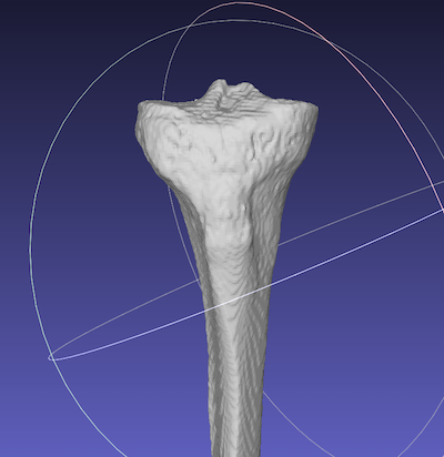
The surface data of the knee joint is extracted in Meshlab, and saved as “joint.stl”.
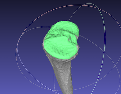
Green:”joint.stl”
import numpy as np
import fitting
from stl import mesh #use numpy-stl
joint_stl = mesh.Mesh.from_file('joint.stl')
point_list = joint_stl.points.reshape([-1, 3])
v, com = fitting.fit_plane(point_list)
print(v)
[ 0.26270565 -0.32178232 0.90963835]
print(com)
[ -42.37019 -38.650146 1169.6364 ]
Confirm the results by a program to draw a plane with given point and normal vector.
fitting.draw_plane(v, com)※ function “draw_plane” is shown later.
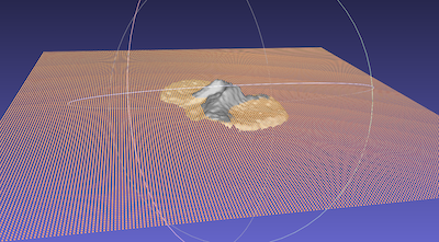
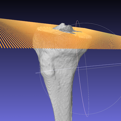
A plane is fit on the joint surface.
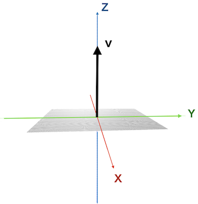
“Draw a Plane” Script
Let’s write a python script to create a plane of points cloud with given vector and point.
Set point cloud on xy plane (z = 0)
↓
Point cloud is rotated \(\theta\) around the Y axis, then rotated \(\phi\) around the Z axis.
The \(\theta\) and \(\phi\) are calculated from the normal vector of the plane.
↓
Rotate the point cloud by rotation matrices calculated from \(\theta\) and \(\phi\).
↓
Translate the point clouds with the center of mass.
The normal vector can be set by
rotating unit vector on the Z axis \(\theta\) around Y axis and \(\phi\) around Z axis.
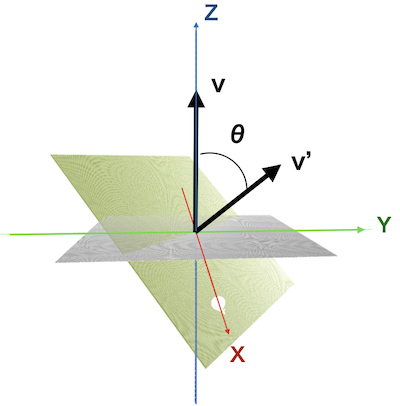
Rotate the Z unit vector \(\theta\) around the Y axis.
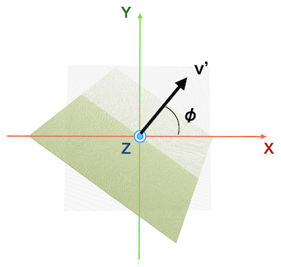
View from above xy plane. Rotate the vector \(\phi\) around the Z axis.
The length of the normal vector is set as r.
(r = 1 in definition)
x, y, z values of \(v’\) are
\(z = r \cos\theta\)
\(y = r \sin\theta \sin\phi\)
\(x = r \sin\theta \cos\phi\)
The angles can be calculated.
\(\theta = \displaystyle \frac {z}{r} \arccos \theta\)
\(\phi = atan2 (y, x)\)
※ atan2 (x1, x2) is the angle consists of x1 in y-axis and x2 in x-axis directions.
\(tan\theta = \displaystyle \frac {x1}{x2}\)
3×3 Rotation matrix of \(\theta\) rotation around the Y axis is
\(
\begin{pmatrix}
\cos \theta & 0 & \sin \theta \\
0 & 1 & 0 \\
-\sin \theta & 0 & \cos \theta
\end{pmatrix}\)
3×3 Rotation matrix of \(\theta\) rotation around the Z axis is
\(
\begin{pmatrix}
\cos \phi & – \sin \phi & 0 \\
\sin \phi & \cos \phi & 0 \\
0 & 0 & 1
\end{pmatrix}\)
After rotation by these matrices,
the point cloud is translated by – com (center of mass) vector.
In Python script,
def draw_plane(plane_v, com, plane_asc_name='plane.asc', d=100):
    """
    input
        plane_v : the normal vector
        com : xyz of center of mass
        plane_asc_name : file name for point cloud, default:'plane.asc'
        d : draw the plane from -d to d, default: 100
    """
    point_cloud = []
    # draw point cloud from -d to d on the xy plane
    for i in range(-d, d):
        for j in range(-d, d):
            point_cloud.append(np.array([i, j, 0]))
    point_cloud = np.array(point_cloud)

    # rotate the point cloud theta around the y-axis, phi the z-axis
    theta = np.arccos(plane_v[2] / np.linalg.norm(plane_v))
    phi = np.arctan2(plane_v[1], plane_v[0])

    # calculate 3x3 rotation matrix to rotate the Z unit vector to the normal vector
    rotation_y = np.array([[np.cos(theta), 0, np.sin(theta)],
                           [0, 1, 0],
                           [-np.sin(theta), 0, np.cos(theta)]])
    rotation_z = np.array([[np.cos(phi), -np.sin(phi), 0],
                           [np.sin(phi), np.cos(phi), 0],
                           [0, 0, 1]])
    rotation_matrix = np.dot(rotation_z, rotation_y)
    # rotate the point cloud by 3x3 matrix, using numpy broadcasting
    translated_points = np.dot(rotation_matrix, point_cloud.T).T + com
    # save the point cloud in ".asc" for Meshlab
    np.savetxt('plane.asc', translated_points)

    return
Principle of Fitting a Plane
Least Square and Constraint
Why the best fit plane is calculated from eigenvector?
The equation for a plane is represented as
\(ax + by + cz = h\)
by setting
\(t = (a, b, c)\)
It equals to
\(t \cdot p = h\)
defining the normal’s length as 1
\(\| \boldsymbol{t} \| = 1\)
For point cloud
\(p_i\) (i = 0 to n),
Least Square Method is used.
The best fit plane is the plane makes the sum of distance from the point cloud minimized.
The best fit plane minimized the cost function,
\(f(t, h) = \displaystyle \sum_i (t \cdot p_i \ – h)^2\)
\(t\): the normal vector
because the length of t equals to 1
\(\| \boldsymbol{t} \| = 1\)
\(g(t, h) = t \cdot t – 1 = 0\)
is a constraint for \(f(t, h)\)
In such a condition,
Method of Lagrange Multipliers
can be used.
Method of Lagrange Multipliers
To minimize or maximize
\(f(x, y)\)
with constraint of
\(g(x, y) = 0\),
defining
\(F(x, y) = f(x, y) + \lambda g(x, y)\),
x, y, \(\lambda \)
satisfy
\(\displaystyle \frac{\partial F}{\partial x} = \displaystyle \frac{\partial F}{\partial y} = \displaystyle \frac{\partial F}{\partial \lambda} = 0 \)
The best fit plane passes the center of mass
Applying this Langrange multipliers method,
\(F(t, h)\) is set as
\(F(t, h) = f(t, h) – \lambda g(t, h)\)
\( = \displaystyle \sum_i (t \cdot p_i \ – h)^2 – \lambda (t \cdot t – 1)\)
At first,
\(\displaystyle \frac{\partial F}{\partial h} = 0\)
can be solved.
\(\displaystyle \frac{\partial F}{\partial h} = 2(t \cdot \displaystyle \sum_i p_i \ – N h) = 0\)
\(h = t \cdot \displaystyle \frac {1}{N}\displaystyle \sum_i p_i\)
Here,
\(\displaystyle \frac {1}{N}\displaystyle \sum_i p_i\)
equals to center of mass of the point cloud,
from the equation
\(t \cdot p = h\)
The best fit plane passes the center of mass.
Eigenvector and eigenvalue satisfy the equation
To simplify the equation,
substitute the values of the center of mass
\(com = \displaystyle \frac {1}{N}\displaystyle \sum_i p_i\)
\(q_i = p_i – com\)
\(h = 0\)
\(f(t)\) is
\(f(t) = \displaystyle \sum_i (t \cdot q_i)^2\)
\(F(t,\lambda)\) is
\(F(t,\lambda) = \displaystyle \sum_i (t \cdot q_i)^2 – \lambda(t \cdot t – 1)\)
Solve the next equation,
\(\displaystyle \frac{\partial F}{\partial t} = 0 \)
\(\displaystyle \frac{\partial F}{\partial t} = 2 \displaystyle \sum_i q_i(t\cdot q_i) – 2\lambda t\) = 0
Here, the formula of the vector inner product
\(a (b \cdot c) = (a \cdot b^{\mathrm{T}}) \cdot c \)
\(\displaystyle \frac{\partial F}{\partial t}\) is
\(\displaystyle \sum_i q_i \cdot q_i^{\mathrm{T}} t – \lambda t = 0\)
By setting 3×3 matrix Q as
\(Q = \displaystyle \sum_i q_i \cdot q_i^{\mathrm{T}}\)
\(Q \cdot t – \lambda t = 0\)
\(t\) and \(\lambda \) which satisfy this equation,
are
Eigenvectors and Eigen Values of 3×3 matrix \(Q\)
In summary,
when \(t\) is the eigenvector of \(Q\),
\(\displaystyle \frac{\partial F}{\partial t} = 0 \)
and
\(f(t) = \displaystyle \sum_i (t \cdot q_i)^2\)
gives extremum (maximum or minimum)
Eigenvector of the minimum eigenvalue is the normal axis
Which eigenvector minimizes the \(f(t)\)?
Substitute
\(t = v\) \(v\): eigenvector
into
\(f(t) = \displaystyle \sum_i (t \cdot q_i)^2\)
\(= t^{\mathrm{T}} \displaystyle \sum_i \cdot q_i \cdot q_i^{\mathrm{T}} \cdot t\)
Here, substitute
\(Q = \displaystyle \sum_i q_i \cdot q_i^{\mathrm{T}}\)
\(f(t) = v \cdot (Q \cdot v)\)
\(v\) and \(\lambda\) satisfy
\(Qv = \lambda v\)
So,
\(f(t) = v \cdot (\lambda v)\)
\(= \lambda \|v\|^2 \)
\(= \lambda\)
because \(\|v\|^2 = 1\)
when
\(\displaystyle \frac{\partial F}{\partial t} = 0 \) ,
\(Q =\) eigenvalue
among eigenvectors,
The eigenvector of the minimum eigenvalue
is the normal vector of the best fit plane.