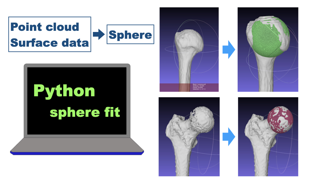
Some joint bones have spherical shape.
Such as
- Humeral head in the shoulder joint
- Femoral head in the hip joint
To describe motion or morphology of these joints, calculating the parameters like radius and center is important.
Calculation process is a little complex.
So, you can understand from
“Python script for sphere fitting” session
=>”Python script for sphere fitting”
Calculation process of sphere fitting
The sphere fit on point clouds is calculated by
“Least Squares Method”
We set the radius and center of the sphere, and point cloud.
\(r\) : radius
\(m\) : center point
\(v_k\) : point vectors of the point clouds
Here, we try to minimize cost function
\(C = \displaystyle \sum_{k=1}^{n}\left\lbrace (v_k – m)^2 – r^2 \right\rbrace ^2 \)
The cost function is differentiated with respect to \(r\) and \(m\).
Differentiation with respect to \(r\) provides
\(-4r \displaystyle \sum_{k=1}^{n}\left\lbrace (v_k – m)^2 – r^2 \right\rbrace = 0 \)
Because \(r \neq 0 \)
\(r = \sqrt{\displaystyle \frac{1}{N}\sum_{k=1}^{n}(v_k – m)^2}\) ・・・ ①
Differentiation with respect to \(m\) provides
\(\displaystyle \sum_{k=1}^{n}(v_k – m)\left\lbrace (v_k – m)^2 – r^2 \right\rbrace = 0\)
substitute \(r\) from the formula ①
\(\displaystyle \frac{1}{N}\sum_{k=1}^{n}v_k^3 – \displaystyle\frac{1}{N}\sum_{k=1}^{n}v_k \cdot \displaystyle\frac{1}{N}\sum_{k=1}^{n}v_k^2 – 2 \left\lbrace \displaystyle \frac{1}{N}\sum_{k=1}^{n} v_k(v_k \cdot m) – \displaystyle\frac{1}{N}\sum_{k=1}^{n}v_k (m \cdot \displaystyle\frac{1}{N}\sum_{k=1}^{n}v_k)\right\rbrace \) = 0
multiplier and mean are aligned by defining
\(\displaystyle \frac{1}{N}\sum_{k=1}^{n}v_k^3 = \overline{v_k^3}\)
\(\displaystyle \frac{1}{N}\sum_{k=1}^{n}v_k^2 = \overline{v_k^2}\)
\(\displaystyle \frac{1}{N}\sum_{k=1}^{n}v_k = \overline{v_k}\)
,
\(\overline{v_k^3} – \overline{v_k}(\overline{v_k^2}) = 2\left\lbrace \displaystyle \frac{1}{N}\sum_{k=1}^{n} v_k(v_k \cdot m) – \overline{v_k} (m \cdot \overline{v_k})\right\rbrace \)
Here,
\(a (b \cdot c) = (a \cdot b^{\mathrm{T}}) \cdot c \)
※ Vector is longitudinal [1, 3] array,
\( (a \cdot b^{\mathrm{T}})\) is 3×3 matrix
for example,
\(
a =
\left(
\begin{array}{c}
a_1 \\
a_2 \\
a_3
\end{array}
\right)
\) \(
b =
\left(
\begin{array}{c}
b_1 \\
b_2 \\
b_3
\end{array}
\right)
\)
then,
\(a \cdot b^{\mathrm{T}} =
\left(
\begin{array}{ccc}
a_1b_1 & a_1b_2 & a_1b_3\\
a_2b_1 & a_2b_2 & a_2b_3 \\
a_3b_1 & a_3b_2 & a_3b_3
\end{array}
\right)
\)
Using this formula,
by setting
\( A = 2\left( \displaystyle \frac{1}{N}\sum_{k=1}^{n} v_k \cdot v_k^{\mathrm{T}} – \overline{v_k} \cdot \overline{v_k}^{\mathrm{T}}\right) \) ・・・ ②
\(b = \overline{v_k^3} – (\overline{v_k^2})\overline{v_k}\) ・・・・・・ ③
provides,
\(A \cdot m = b\)
Overall,
\(m = A^{-1} \cdot b\)
radius \(r\) and
center \(m\)
are calculated.

Fit a sphere by python script
For point vector of the point cloud: \(v\)
calculate radius:\(r\)
from
\(r = \sqrt{\displaystyle \frac{1}{N}\sum_{k=1}^{n}(v_k – m)^2}\) ・・・①
By calculating
\(\displaystyle \frac{1}{N}\sum_{k=1}^{n}v_k^3 = \overline{v_k^3}\)
\(\displaystyle \frac{1}{N}\sum_{k=1}^{n}v_k^2 = \overline{v_k^2}\)
\(\displaystyle \frac{1}{N}\sum_{k=1}^{n}v_k = \overline{v_k}\)
\( A = 2\left( \displaystyle \frac{1}{N}\sum_{k=1}^{n} v_k \cdot v_k^{\mathrm{T}} – \overline{v_k} \cdot \overline{v_k}^{\mathrm{T}}\right) \) ・・・ ②
\(b = \overline{v_k^3} – (\overline{v_k^2})\overline{v_k}\) ・・・・・・ ③
from
\(A \cdot m = b\)
,
center \(m\) is calculated.
Write down those process in python script.
file name is
“fitting.py”
def sphere_fit(point_cloud):
    """
    input
        point_cloud: xyz of the point clouds numpy array
    output
        radius : radius of the sphere
        sphere_center : xyz of the sphere center
    """

    A_1 = np.zeros((3,3))
    #A_1 : 1st item of A
    v_1 = np.array([0.0,0.0,0.0])
    v_2 = 0.0
    v_3 = np.array([0.0,0.0,0.0])
    # mean of multiplier of point vector of the point_clouds
    # v_1, v_3 : vector, v_2 : scalar

    N = len(point_cloud)
    #N : number of the points

    """Calculation of the sum(sigma)"""
    for v in point_cloud:
        v_1 += v
        v_2 += np.dot(v, v)
        v_3 += np.dot(v, v) * v

        A_1 += np.dot(np.array([v]).T, np.array([v]))

    v_1 /= N
    v_2 /= N
    v_3 /= N
    A = 2 * (A_1 / N - np.dot(np.array([v_1]).T, np.array([v_1])))
    # formula ②
    b = v_3 - v_2 * v_1
    # formula ③
    sphere_center = np.dot(np.linalg.inv(A), b)
    # formula ①
    radius = (sum(np.linalg.norm(np.array(point_cloud) - sphere_center, axis=1))
              /len(point_cloud))

    return(radius, sphere_center)
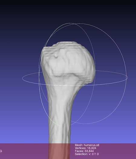
Example to use the python program(humeral head)
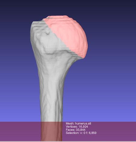
A sphere is fit on the humeral head.
the surface of the humeral head is extracted by Meshlab
and saved as
“sphere.stl”.
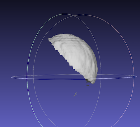
fitting a sphere is performed in python interpreter by using ‘fitting.py’.
import numpy as np
import fitting

from stl import mesh
# use numpy-stl to manipulate surfaces

sphere_stl = mesh.Mesh.from_file('sphere.stl')
# read stl file
sphere_points = sphere_stl.points.reshape([-1, 3])
# read point clouds of the stl
print(sphere_points)

# [[ 154.80566  -124.725586  192.21085 ]
# [ 153.9873   -124.725586  192.33838 ]
# [ 153.9873   -124.098175  193.5     ]
# ...
# [ 157.29794  -124.725586  235.5     ]
# [ 157.26074  -124.711945  235.5     ]
# [ 157.26074  -124.725586  235.52    ]]
# point vectors of the point clouds

radius, center = fitting.sphere_fit(sphere_points)
# calculate by sphere_fit function in fitting.py
print(radius)
# 23.087794980492543
print(center)
# [ 154.15674832 -133.40106545  213.64071843]
the radius and center are calculated.
Let’s confirm these result by draw a sphere with the stl file.
Draw a sphere by setting radius and center
add a script in “fitting.py” to draw a sphere for Meshlab.
"""create point clouds by inputting radius and center"""
def draw_sphere(radius, sphere_center):
    """
    inpu
        radius:radius (scalar)
        sphere_center : xyz of the sphere center (numpy array)
    """

    point_list = []

    """create point_cloud"""
    for i in range(360):
        i = i * np.pi / 180   # use radian
        for j in range(360):
            j = j * np.pi / 180  # use radian
            point = radius * np.array([np.sin(i) * np.cos(j),np.sin(i) * np.sin(j), np.cos(i)]) + sphere_center
            # adding a point on the sphere
            point_list.append(point)

    point_list = np.array(point_list)
    # data are stored in numpy array type
    np.savetxt('sphere.asc', point_list)
    # save as '.asc' file for Meshlab
    return
In python interpreter,
fitting.draw_sphere(radius, sphere_center)
# radius, sphere_center are the values have been calculated.
“sphere.asc” is saved.
This file can be opened in Meshlab.
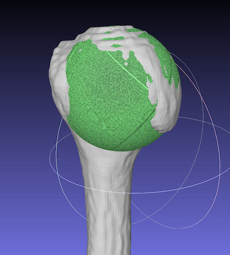
a sphere was fit on the humeral head well.