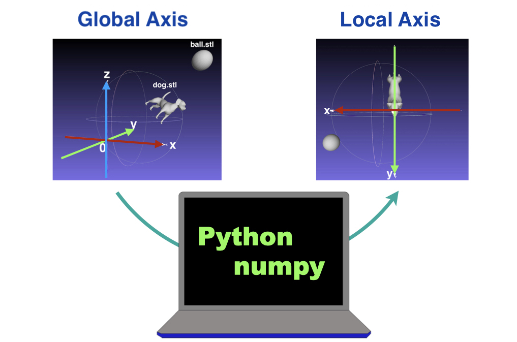
Coordinate System – Global and Local axes –

Coordinate systems – Global and Local axes –

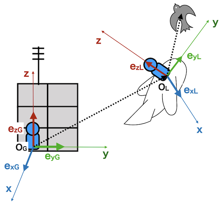
Here is an example of two coordinate systems

A passenger on a airplane
A person on the ground

Let’s describe
position of a bird
from these two viewpoints.

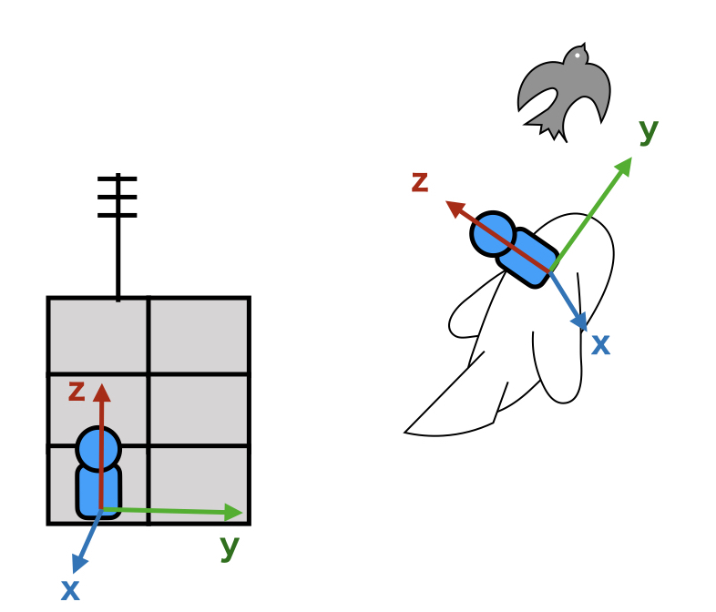
There are two coordinate systems on the airplane and the ground.
The position of a subject is described individually by each coordinate systems (xyz axes).
Generally,
coordinate systems of the reference axis is called as
Global Axis
and the moving axis is called as
Local Axis.

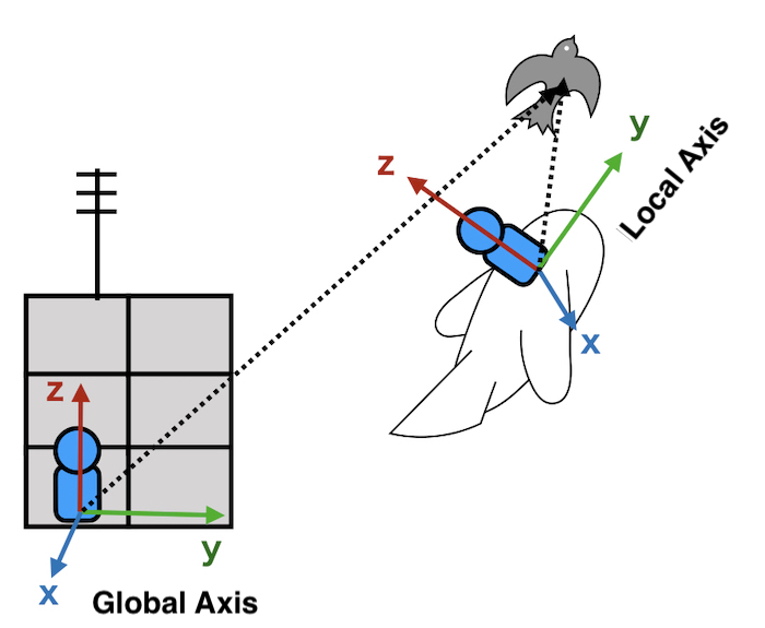
So, here we define
ground　＝> Global Axis
Airplane ＝> Local Axis

Position in the local axis

Let’s go back to the bird position.

The bird position is
\((x_L, y_L, z_L)\)
in the local axis.

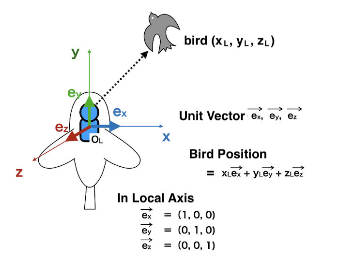
from the origin in the local axis \(O_L\)

the position vector of the bird is

\(x_L\overrightarrow{e_x} + y_L\overrightarrow{e_y} + z_L\overrightarrow{e_z}\)

Of course,

\(\overrightarrow{e_x} = (1, 0, 0)\)
\(\overrightarrow{e_y} = (0, 1, 0)\)
\(\overrightarrow{e_z} = (0, 0, 1)\)

Local Axis to Global Axis

Let’s calculate the bird position in the Global Axis.

Each coordinate system has unit vectors of xyz as

\(\overrightarrow{e_x}, \overrightarrow{e_y}, \overrightarrow{e_z}\)

The unit vectors in the local axis have x, y, z values in the global axes because the airplane is rotated.

 

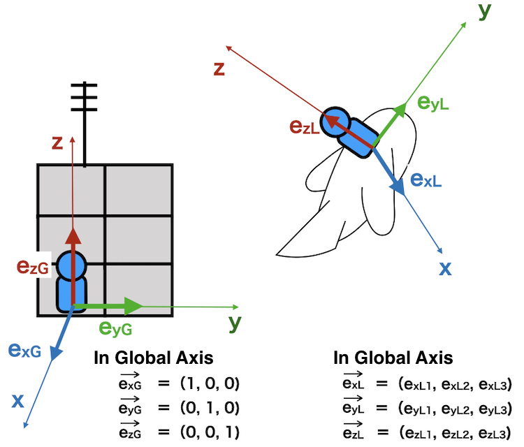
such as

\(\overrightarrow{e_{xL}} = (e_{xL1}, e_{xL2}, e_{xL3})\)
\(\overrightarrow{e_{yL}} = (e_{yL1}, e_{yL2}, e_{yL3})\)
\(\overrightarrow{e_{zL}} = (e_{zL1}, e_{zL2}, e_{zL3})\)

The bird position
\((x_G, y_G, z_G)\) in global axis
for \((x_L, y_L, z_L)\) in local axis,

 
\(x_L\overrightarrow{e_{xL}} + y_L\overrightarrow{e_{yL}} + z_L\overrightarrow{e_{zL}} + \overrightarrow{O_GO_L} \)

equals to
inner product between
matrix consists of 3 unit vectors and
position vector in local coordinate system.

\(
\left(
\begin{array}{c}
x_G \\
y_G \\
z_G
\end{array}
\right)
=\begin{pmatrix}
e_{xL1} & e_{yL1} & e_{zL1} \\
e_{xL2} & e_{yL2} & e_{zL2} \\
e_{xL3} & e_{yL3} & e_{zL3}
\end{pmatrix}
\left(
\begin{array}{c}
x_L \\
y_L \\
z_L
\end{array}
\right)
+ \overrightarrow{O_GO_L}
\)

This formula can be written by

\(
\left(
\begin{array}{c}
x_G \\
y_G \\
z_G
\end{array}
\right)
= M
\left(
\begin{array}{c}
x_L \\
y_L \\
z_L
\end{array}
\right)
+ t
\)

\(M = \left(
\begin{array}{c}
\overrightarrow{e_{xL}} \\
\overrightarrow{e_{yL}} \\
\overrightarrow{e_{zL}}
\end{array}
\right) ^{\mathrm{T}}
\hspace{10pt}
t = \overrightarrow{O_GO_L}
\)
 
※ \(T\) : Transpose matrix

using
Rotation matrix (M) and Translation vector (t)

import numpy as np
v1 = np.array([1, 2, 3])
v2 = np.array([4, 5, 6])
v3 = np.array([7, 8, 9])

M = np.array([v1, v2, v3])
print(M)
# [[1 2 3]
#  [4 5 6]
#  [7 8 9]]

print(M.T)  #transpose matrix
# [[1 4 7]
#  [2 5 8]
#  [3 6 9]]

Transfromation from Global Axis to Local Axis

Backward calculation can transfrom
the bird position \((x_G, y_G, z_G)\) in global axis
into that in local axis.

Start from the formula

\(
\left(
\begin{array}{c}
x_G \\
y_G \\
z_G
\end{array}
\right)
= M
\left(
\begin{array}{c}
x_L \\
y_L \\
z_L
\end{array}
\right)
+ t
\)

translate by subtracting \(t\)

\(
\left(
\begin{array}{c}
x_G \\
y_G \\
z_G
\end{array}
\right)
– t
= M
\left(
\begin{array}{c}
x_L \\
y_L \\
z_L
\end{array}
\right)
\)
 

multiply \(M^{-1}\) from the left side

 
\(
M^{-1}
\left(
\begin{array}{c}
x_G \\
y_G \\
z_G
\end{array}
\right)
– M^{-1}t
=
\left(
\begin{array}{c}
x_L \\
y_L \\
z_L
\end{array}
\right)
\)
 

Because M is a rotation matrix,

\(M^{-1} = M^{\mathrm{T}}\)

 
Then,

\(
M^{\mathrm{T}}
\left(
\begin{array}{c}
x_G \\
y_G \\
z_G
\end{array}
\right)
– M^{\mathrm{T}}t
=
\left(
\begin{array}{c}
x_L \\
y_L \\
z_L
\end{array}
\right)
\)
 

Rotation Matrix is

 
\(M^{\mathrm{T}} = \left(
\begin{array}{c}
\overrightarrow{e_{xL}} \\
\overrightarrow{e_{yL}} \\
\overrightarrow{e_{zL}}
\end{array}
\right)
\hspace{10pt}
\)
 
Translation vector is

\(
– M^{\mathrm{T}} \cdot \overrightarrow{O_GO_L}
\)

Transformation matrix 4×4 includes rotation and translation

Rotation and translation can be described by
a 4×4 transformation matrix.

When the point clouds are moved,
the process is divided into
Rotation and Translation.

Rotation is described 3×3 matrix.
Translation is described xyz vector.

Here, rotation matrix
\(Rot=
\begin{pmatrix}
r_{11} & r_{12} & r_{13} \\
r_{21} & r_{22} & r_{23} \\
r_{31} & r_{32} & r_{33}
\end{pmatrix}\),

Translation matrix
\(t = \left(
\begin{array}{c}
t_x \\
t_y \\
t_z
\end{array}
\right)\)

 
When a point \(pi\) is

\(pi=\left(
\begin{array}{c}
p_{ix} \\
p_{iy} \\
p_{iz}
\end{array}
\right)\)

,

transformed point is

\(Rot \cdot p_i + t\)

,
Here we add one 1 element to \(pi\)

 
\(pi=\left(
\begin{array}{c}
p_{ix} \\
p_{iy} \\
p_{iz} \\
1
\end{array}
\right)\)
 

Then we apply 4×4 matrix
 
\(R=
\left(
\begin{array}{ccc|c}
& & &\\
& \Large{Rot} & & \large{t}\\
& & & \\
\hline
& \large{0} & & \large{1}
\end{array}
\right)
\)
 
the elements of the matrix are
 

\(
R \cdot pi =
\begin{pmatrix}
r_{11} & r_{12} & r_{13} & t_x\\
r_{21} & r_{22} & r_{23} & t_y\\
r_{31} & r_{32} & r_{33} & t_z\\
0 & 0 & 0 & 1
\end{pmatrix}
\cdot
\left(
\begin{array}{c}
p_{ix} \\
p_{iy} \\
p_{iz} \\
1
\end{array}
\right)
=
\left(
\begin{array}{c}
\\
Rot \cdot pi + t \\
\\
1
\end{array}
\right)\)

We can calculate the transformed point by
one time inner product.
 

  

Caution!!　4×4 inverse matrix is not inverse transformation !!

In 3×3 rotation matrix,

\(^{L}Rot_G = (^{G}Rot_L) ^{-1}\)

inverse matrix = inverse rotation

but in 4×4 transformation matrix contains

rotation　⇒　translation

This inverse transformation is

translation　⇒　rotation

Then, inverse transformation of 4×4 matrix

\(\left(
\begin{array}{ccc|c}
& & &\\
& \Large{Rot} & & \large{t}\\
& & & \\
\hline
& \large{0} & & \large{1}
\end{array}
\right)\)

is

\(\left(
\begin{array}{ccc|c}
& & &\\
& \Large{Rot^{-1}} & & – Rot^{-1} \cdot {t}\\
& & & \\
\hline
& \large{0} & & \large{1}
\end{array}
\right)\)

This is not equal to the inverse matrix.